The Mediterranean Forecasting System is a coupled hydrodynamic-wave model with data assimilation components. The model horizontal grid resolution is 1/16˚ (6-7 km, approximately) and it is resolved over 72 unevenly spaced vertical levels. It is nested to the Atlantic ocean through the Copernicus global ocean analyses and forecasts (https://marine.copernicus.eu).The wave model uses 24 directional bins (15° directional resolution) and 30 frequency bins (ranging between 0.05Hz and 0.7931 Hz) to represent the wave spectra distribution.
The Nucleus for European Modelling of the Ocean [6,7] (NEMO,https://www.nemo-ocean.eu) is used for the hydrodynamics component and WaveWatch-III [8] (https://polar.ncep.noaa.gov/waves/index2.shtml) for the wave component.
Ocean measurements from satellites (SLA) and in situ (temperature and salinity from ARGO floats, CTD and XBT) are assimilated on a daily basis, following a weekly cycle of assimilation. The following table presents the main characteristics of the two systems.
| COSMO MFS | ECMWF MFS | |
| Version | EAS1_COSMO_SYS | EAS1_ECMWF_SYS |
| Model | NEMO v3.4 + WWIII v3.14 | NEMO v3.4 + WWIII v3.14 |
| Horizontal res. | 1/16° x 1/ 16° (~ 6 – 7 km) | 1/16° x 1/ 16° (~ 6 – 7 km) |
| Vertical res. | 72 z (partial steps) | 72 z (partial steps) |
| Atmospheric Forcing | COSMO-ME 1/16° (~ 6 – 7 km) | ECMWF 1/8 (~ 13 km) |
| Initial Condition | 21-May-2019 Restart file from ECMWF MFS | 1-Jan-2011 Climatology from SeaDataNet |
| Boundary Conditions | GLO-MFC daily data sets 1/12° hor. res. | GLO-MFC daily data sets 1/12° hor. res. |
| Assimilation scheme | OceanVAR 3dVAR | OceanVAR 3dVAR |
| Assimilated data | SLA (Jason1, Jason2, Altika, Cryosat, Envisat), in situ T/S profiles | SLA (Jason1, Jason2, Altika, Cryosat, Envisat), in situ T/S profiles |
| Atmospheric pressure | Yes | Yes |
| Free-surface formulation | Split explicit | Split explicit |
| Horizontal eddy diffusivity coeff. for tracers | -6.e^8 [m4/s] | -6.e^8 [m4/s] |
| Horizontal bilaplacian eddy viscosity coeff. | -1.e^9 [m4/s] | -1.e^9 [m4/s] |
| Time step | 300 s | 300 s |
Model
Hydrodynamic and wave numerical model components
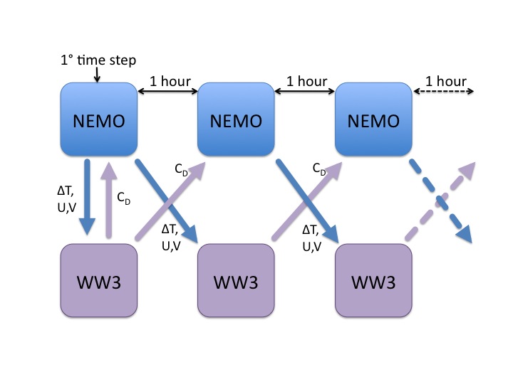
NEMO for the hydrodynamics and WWIII for the waves have been implemented in the Mediterranean Sea at 1/16° x 1/16° horizontal resolution. The hydrodynamic model provides estimates of air-sea temperature difference and surface currents to the wave model, which returns back to the hydrodynamics the neutral component of the surface drag coefficient, taking into account the wave induced effect at the air-sea interface. The coupling between the hydrodynamics and the waves is implemented as shown in the following scheme [9].
Figure 2: Scheme of the current-wave coupling
The NEMO code solves the primitive equations using the linear free surface formulation and it uses vertical partial cells to best fit the bottom topography. Seven rivers are considered as volume input: Ebro, Rhone, Po, Vjose, Seman, Bojana and Nile, moreover the Dardanelles Strait is closed but considered as a river in terms of net volume source.
The WWIII model solves the wave action balance equation in slowly varying depth domain, considering a superposition of the following source/sink terms: wind input growing action based on Janssen’s quasi-linear theory of wind-wave generation [10,11], a dissipation source term [12], whitecapping theory [13] and nonlinear resonant wave-wave interactions modelled using the Discrete Interaction Approximation (DIA) [14,15]. The spectral discretization is obtained through 30 frequency bins ranging from 0.05 Hz (20 s) to 0.79 Hz (1.25 s) and 24 equally distributed directional bins.
Data Assimilation
The data assimilation system is a variational scheme [16,17,18] developed with a specific background error correlation matrix formulation. The assimilated data include: sea level anomaly, in situ temperature profiles from VOS XBTs (Voluntary Observing Ship-eXpandable BathyThermograph), in situ temperature and salinity profiles from ARGO floats, and in situ temperature and salinity profiles from CTD and gliders. Satellite objectively analyzed Sea Surface Temperature is used for the correction of surface heat fluxes.
All the assimilated observations are provided by the Thematic Assembly Centers of Copernicus (https://marine.copernicus.eu/).
Cal/Val system
The quality assessment of the system is monitored weekly by the calculation of the root mean square statistics of difference between observations and model background fields (so-called misfits):
- https://medforecast.bo.ingv.it/cosmo-mfs-evaluation/
- https://medforecast.bo.ingv.it/ecmwf-mfs-evaluation/
The systems performance is also evaluated by considering independent data at fixed stations around the Mediterranean Sea and results are displayed here: https://calval.bo.ingv.it
Production Cycle
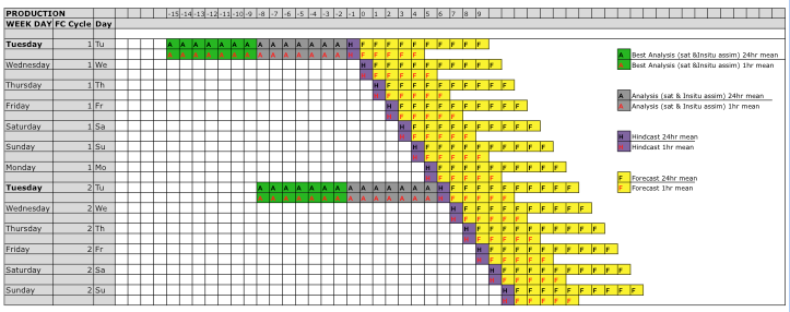
Analysis are produced weekly, on Tuesdays, for the previous 14 days. The assimilation cycle is performed on a daily basis and it runs in filtered mode. In the ECMWF MFS two products are available with a different frequency of output. A 10-day forecast is produced as daily means whereas a 5-day forecast has an hourly output frequency. In the COSMO MFS a 3-day forecast is produced both with hourly and daily output.
Each forecast is initialized by a hindcast every day except for Tuesday, when the analysis is used instead. The production cycle of ECMWF MFS is represented here below.
Products
| COSMO MFS | ECMWF MFS | |
| Geographical coverage | 6° W — 36.25° E 30.187°N — 45.937° N | 15° W — 36.25° E 30.187°N — 45.937° N |
| Variables | * Potential Temperature * Salinity * Sea Surface Height * Horizontal current velocity (meridional and zonal components) * Wind stress (meridional and zonal components) * Net upward Water Flux * Net Downward heat Flux * Shortwave Radiation * Vertical eddy diffusivity * Surface Stokes Drift velocity (meridional and zonal components) * Significant wave height * Wave mean period * Wave peak period * Mean wave direction * Mean wind direction * Mean wave number * Mean wave length * Drag coefficient * Friction velocity (module) | * Potential Temperature * Salinity * Sea Surface Height * Horizontal current velocity (meridional and zonal components) * Wind stress (meridional and zonal components) * Net upward Water Flux * Net Downward heat Flux * Shortwave Radiation * Vertical eddy diffusivity * Surface Stokes Drift velocity (meridional and zonal components) * Significant wave height * Wave mean period * Wave peak period * Mean wave direction * Mean wind direction * Mean wave number * Mean wave length * Drag coefficient * Friction velocity (module) |
| Analysis | Yes | Yes |
| Hindcast | Yes | Yes |
| Forecast | Yes | Yes |
| Nominal start of forecast / length of forecast | 12:00 UTC / 240 h | 12:00 UTC / 240 h |
| Available time series | * 24 h average fields: from 28-May-2019 — ongoing * 1 h average fields: 1 month rolling archive * 1 h instant wave fields: 1 month rolling archive | * 24 h average fields: from 1-Jan-2013 — ongoing * 1 h average fields: 1 month rolling archive * 1 h instant wave fields: 1 month rolling archive |
| Temporal resolution | * 24 h average fields * 1 h average fields * 1 h instant wave fields | * 24 h average fields * 1 h average fields * 1 h instant wave fields |
| Target production time | * Forecast: daily at 01:00 UTC of the day+1 from nominal start of forecast * Analysis: Wednesday, 01:00 UTC of the day+1 from nominal start of forecast * Hindcast: daily at 01:00 UTC of the day+1 from nominal start of forecast | * Forecast: daily at 01:00 UTC of the day+1 from nominal start of forecast * Analysis: Thursday 01:00 UTC of the day+1 from nominal start of forecast * Hindcast: daily at 01:00 UTC of the day+1 from nominal start of forecast |
| Delivery mechanism | Not delivered | Not delivered |
| Horizontal resolution | 1 / 16 ° | 1 / 16 ° |
| Number of vertical levels | 72 | 72 |
| Format | netCDF-4 (CF 1.6) | netCDF-4 (CF 1.6) |
References
[1] Pinardi, N., I. Allen, P. De Mey, G. Korres, A. Lascaratos, P.Y. Le Traon, C. Maillard, G. Manzella and C. Tziavos, 2003. The Mediterranean ocean Forecasting System: first phase of implementation (1998-2001). Ann. Geophys., 21, 1, 3-20
[2] Roullet G. and G. Madec, 2000: Salt conservation, free surface, and varying levels: a new formulation for ocean general circulation models. J.G.R., 105, C10, 23,927-23,942
[3] Tonani, M., N. Pinardi, S. Dobricic, I. Pujol, and C. Fratianni, 2008. A high-resolution free-surface model of the Mediterranean Sea. Ocean Sci., 4, 1-14
[4] Tonani M., N.Pinardi, M.Adani, A. Bonazzi, G.Coppini, M.De Dominicis, S.Dobricic, M.Drudi, N.Fabbroni, C.Fratianni, A.Grandi, S.Lyubartsev, P.Oddo, D. Pettenuzzo, J. Pistoia and I. Pujol, 2008. The Mediterranean ocean Forecasting System. Proceedings of the Fifth International Conference on EuroGOOS 20-22 May 2008, Exeter, UK, edited by H. Dahlin, EuroGOOS Office, Norrkoping, Sweden, M. J. Bell, Met Office, UK, N. C. Fleming, UK, S. E. Pietersson, EuroGOOS Office, Norrkoping, Sweden. First Published 2010, EuroGOOS Publication no.28, ISBN 978-91-974828-6-8
[5] Oddo P., M. Adani N. Pinardi, C. Fratianni, M. Tonani, D. Pettenuzzo, 2009. A Nested Atlantic-Mediterranean Sea General Circulation Model for Operational Forecasting. Ocean Sci. Discuss., 6, 1093-1127
[6] Dombrowsky E., L. Bertino, G.B. Brassington, E.P. Chassignet, F. Davidson, H.E. Hurlburt, M. Kamachi, T. Lee, M.J. Martin, S. Meu and M. Tonani 2009: GODAE Systems in operation, Oceanography, Volume 22-3, 83,95 NEMO ocean engine, Note du Pole de modelisation, Institut Pierre-Simon Laplace (IPSL), France, No 27 ISSN No 1288-1619
[7] Madec, G., P. Delecluse, M. Imbard and C. Levy, 1998. OPA version 8.1 ocean general circulation model reference manual. Technical Report, LODYC/IPSL, Note 11, pp 91
[8] Madec, G., 2008. NEMO ocean engine. Note du Pole de modélisation, Institut Pierre-Simon Laplace (IPSL), France, Note 27 ISSN 1288-1619, pp 209
[9] Tolman H.L., 2009. User Manual and system documentation of WAVEWATCH III version 3.14. NOAA/NWS/NCEP/MMAB Technical Note 213, pp 33
[10] Clementi, E., P. Oddo, M. Drudi, N. Pinardi, G. Korres, A. Grandi, 2017. Coupling hydrodynamic and wave models: first step and sensitivity experiments in the Mediterranean Sea. Ocean Dynamics (2017) 67: 1293. https://doi.org/10.1007/s10236-017-1087-7
[11] Janssen PAEM, 1989. Wave induced stress and the drag of air flow over sea wave, J. Phys. Ocean., 19, 745-754,
[12] Janssen PAEM, 1989. Quasi-Linear theory of wind wave generation applied to wave forecasting, J. Phys. Ocean., 21, 1631-1642, 1991.
[13] Hasselmann, K., 1974. On the characterization of ocean waves due to white capping, Boundary-Layer Meteorology, 6, 107-127, 1974
[14] Komen G.J., S. Hasselmann, K. Hasselmann, 1984. On the existence of a fully developed windsea spectrum. J Phys Oceanogr 14:1271–1285
[15] Hasselmann, S. and Hasselmann, K., 1985: Computations and parameterizations of the nonlinear energy transfer in a gravity wave spectrum. Part I: A new method for efficient computations of the exact nonlinear transfer integral, J. Phys. Ocean., 15, 1369-1377
[16] Hasselmann, S., K. Hasselmann, J. H. Allender, and Barnett, T.P., 1985: Computations and parameterizations of the nonlinear energy transfer in a gravity wave spectrum. Part II: Parameterizations of the nonlinear energy transfer for application in wave models, J. Phys. Ocean., 15, 1378-1391
[17] Dobricic, S. and N. Pinardi, 2008. An oceanographic three-dimensional variational data assimilation scheme. Ocean Modelling, 22, 3-4, 89-105
[18] Dobricic, S., N. Pinardi, M. Adani, M. Tonani, C. Fratianni, A. Bonazzi, and V. Fernandez, 2007. Daily oceanographic analyses by Mediterranean Forecasting System at the basin scale. Ocean Sci., 3, 149-157
[19] Dobricic, S., 2005. New mean dynamic topography of the mediterranean calculated from assimilation system diagnostic. GRL, 32